Recently, my colleague at the thedataist.com published a compelling post about some challenges in machine learning education. You can read it for yourself here, but I’d like to build upon what he posted; it’s bothered me for a long time that the math behind common machine learning algorithms like regression are clouded in confusing mathematical notation.

At its core, machine learning is math. I’m certainly not calling for a complete decoupling of machine learning applications from math. But we as a tech community can probably do a better of mentoring others and helping them understand what’s going on under the hood when they’re applying common machine learning algorithms like linear regression in software packages like scikit-learn.

I’ll attempt to demystify the very useful linear regression method in layman’s terms and Python here. I’ll start by trying to use plain English and intuition, and then going to Python (Pandas and Numpy) to do the heavy data and math lifting. Lastly, I’ll use scikit-learn to show we get the same results using that package.

First, a short glossary:

dependent variable: the variable we’re trying to predict; the variable which depends on some other variable(s). Also known as the target variable or simply, “y“.

independent variable: the variable(s) which can help predict the dependent variable. Also knowns as explanatory variable(s), features, or simply, “X“.

parameter: the amount(s) by which our method increases or reduces the prediction of the dependent variable. Also known as “theta(s)“, “weight(s)“, and “beta(s)“.

error: the distance between our prediction of the dependent variable and the actual dependent variable. Also knows as “residuals“.

model: the entire representation (mathematical or otherwise) of the relationship between the variables, including the parameters

Linear Regression?

Linear regression is a technique used to estimate the relationship between two variables (x and y). The estimated relationship manifests itself in the parameter of X which explains Y. We call it linear because we assume the relationship between the parameters of X and Y to be linear, and not because we assume a strictly linear relationship between X and Y.

A common approach to solve linear regression (to estimate the best parameters of X) is called Ordinary Least Squares (OLS). It’s called that (somewhat awkwardly) because we use it to find the parameter or weight of X that is associated with the least amount of error squared. We use error squared because we’re interested in the distance of our line below from the actual y, and not so much whether it was above or below the line. Also, squaring produces some nice properties that are useful later.

Graphically, this means that if could draw an infinite amount of lines through the dots below, and for each line, sum up all the errors for each line and keep track of them all, the slope of the line which has the least amount of total error associated with it would be the parameter we’re looking for.

This is where things get a little mathy.

Luckily, we don’t have to draw an infinite number of lines and sum up all the error squared to find the slope with the least amount of error. We can solve this problem analytically. We start by identifying an objective function and then use  linear algebra and matrix/vector calculus to do the minimize the function (stay with me!). We’re looking to minimize squared error in our model, so let’s say our objective function is:

(Y – (some_weights * X))²

To simply things, let’s say that Y is a vector (at this point it doesn’t matter if it’s a row or column, so long as your multiplication is consistent) that represents all of our values of the dependent variable y. And X is a vector (or matrix) of the independent variable(s) which we think explain and predict Y. Let’s also say that some_weight is a vector of weights, one for each independent variable in our model.

Remember that when we subtract a vector from a vector, we end up with a vector. So (y – some_weight * x) is a vector. In order to square that vector, we have to transpose one of the vector terms:

(Y – (some_weights * X)^T * (Y – (some_weighs* X)

If we were doing this by hand, we would continue to expand this expression and and set the first derivative (or gradient) of the resulting expression with respect to the unknown parameter (the vector of weights) to zero to solve for it. It turns out that when you do this, you end up with this expression for the parameter estimate.

some_weights  = (X^T X)^-1 * X^TY

As an (important) aside, we would make sure we could invert X^TX and check for a true minimum by taking the second derivative of the expanded expression. I’m going to use Python to check for a true minimum and to estimate the parameter.

Using Python to Estimate the Relationship between Housing Price and Average Number of Rooms

We start by importing Numpy, Pandas and the Boston housing data set and linear_model from scikit-learn.

%matplotlib inline
import numpy as np
import pandas as pd
from sklearn.datasets import load_boston
from sklearn import linear_model
from matplotlib import pyplot as plt

Next we build a full dataframe from all of the Boston housing data. In the Boston data, the price is the target or dependent variable, and the rest are independent or explanatory variables.

boston = pd.DataFrame(load_boston().data, columns=load_boston().feature_names)
boston['target'] = load_boston().target
boston.head()

We’re interested in the relationship between rooms and the price so we plot to see what it looks like graphically:

plt.scatter(boston['RM'], boston['target'])
plt.xlabel('Rooms')
plt.ylabel('Price')
plt.show()

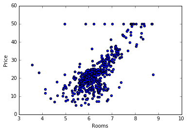
There’s a few funky-looking things going on with the graph, but there’s generally an upward behavior in price (y) as the number of rooms (x) increases. So we can expect for the parameter associated with the X variable to be positive. We also expect to have a vector of weights with only a single value: the parameter associated with number of rooms.

Now we jump right into the math again, but using Python to do the heavy lifting. We’re going to turn the Boston rooms data to Numpy matrix form, starting specifically with column vectors as if we were looking at spreadsheet columns. The rooms data  will be our X. We do the same with the target variable, the house price. This will be our Y:

X = np.matrix(boston['RM']).T
Y = np.matrix(boston['target']).T

Next, using our equation for the unknown parameter (some_weight  = (X^T X)^-1 * X^TY), we declare X^T X and X^TY):

XtX = X.T * X
XtY = X.T * Y

Now all we have to do is make sure we can invert X^T X by checking if the determinant is equal to zero.

np.linalg.det(XtX) == 0

False

Since our matrix was invertible, we can proceed to evaluate the rest of our expression to estimate the unknown parameter (following one convention by calling it w-hat):

w_hat = XtX.I * XtY

We end up with a single parameter for X because we were only estimating a single relationship:

matrix([[ 3.6533504]])

This suggests the target variable increases by 3.65 for every unit increase in the number of rooms. This also validates our graphical intuition that the room number has a positive effect on price.

What happens when we use scikit-learn’s linear regression package?

We declare a model LinearRegression from linear_model and set it to not include an intercept (by default, the package pads the data with a vector of ones) so we can correctly compare our estimate here to our estimate from above.

model = linear_model.LinearRegression(fit_intercept = False)
fit = model.fit(boston['RM'], boston['target'])

This throws an error however, since we’re only using one feature (number of rooms):

/Users/x-macbook-pro/anaconda/lib/python3.5/site-packages/sklearn/utils/validation.py:386: DeprecationWarning: Passing 1d arrays as data is deprecated in 0.17 and willraise ValueError in 0.19. Reshape your data either using X.reshape(-1, 1) if your data has a single feature or X.reshape(1, -1) if it contains a single sample.
  DeprecationWarning)

So let’s follow the tip and reshape our X data:

fit = model.fit(boston['RM'].reshape(-1,1), boston['target'])

Now we can produce the parameter estimate:

fit.coef_

array([ 3.6533504])

As you can see, the more manual Numpy process and the more “black-box” scikit-learn process both produced same exact parameter estimate!

Now go forth, research, and predict.

Here’s a notebook with all the code.